Dynamic modelling
Introduction
Dynamic modelling is modelling of processes over time. In dynamic modelling new attributes are computed as a function of attribute changes over time. After the general concepts (Concepts) are explained, each part of the script will be described, from the structure in the seperate sections of the program (script) for a dynamic model (The script to some special contents of a dynamic modelling script (timeinput, report) and the running of a script (Timeinput and report in the script, running a script). Finally, some examples of dynamic models are given (How to make a dynamic model).
Concepts
Introduction
In a dynamic model, for each timestep a series of pcrcalc operations is consecutively performed using the resulting maps from the previous timestep and/or external data that define the value of an attribute for that timestep. This is done for all timesteps of a model run. Thus a dynamic model can be seen as a temporal sequence of static changes in the state of cells on map(s), each representing the change in the state of the modelled process over the timestep.
In the PCRaster database, the time series covers spatial data that vary over time. For each time step, it contains a set of map cell values that is input or output at that timestep. The format of time series will be described later on (Time series format). Other data used in Dynamic Modelling are the same as used for Cartographic Modelling: the PCRaster map and the table. In a dynamic model a PCRaster map is a variable that may have a different set of cell values for each time step: it is a map that changes in time. A table is used in dynamic modelling to define certain relations between maps. The table must be available in the PCRaster database before a model is run; a table cannot be changed or generated during a model run. The general concept and format of the time series, the PCRaster map en the table has been dicussed earlier (The Database).
The sections of a script
Dynamic models are built with the language provided by PCRaster. Within this language the models can be programmed with the PCRaster operators of Cartographic Modelling. A script, which is a program written in the Dynamic Modelling language, consists of separate sections. Each section contains a certain functional part of the script. The division in sections is an essential concept of the Dynamic Modelling language. It tells the computer how to execute a program and it helps the user to structure the components of a model. The basic sections needed for building a model are the binding section, areamap section, timer section, initial section and the dynamic section. The Table below gives an example of a script for the simulation of the soil water balance. Here, you do not need to know the exact function of the model; it is only given as an idea of a script. The detailed description of the example in the Table will be discussed later on in this chapter (How to make a dynamic model).
Example of a dynamic model.
# model for calculation of reduction in soil moisture content
# incorporated processes: evapotranspiration and infiltration of rain
# timestep one day

binding
 MoistMeas = Moist952.map;
 MoistCrit = scalar(20);
 Eref = scalar(8);
 Kc = CrCoef95.map;
 TimeSeriesMax = Max8.tss;
 TimeSeriesMin = Min8.tss;
 RainTimeSeries = Rain.tss;

areamap
 Clone.map;

timer
 1 30 1;

initial
 report Eact = Kc * Eref;
 Moist = MoistMeas;

dynamic
 Rain = timeinputscalar(RainTimeSeries, 1);
 report Moist = Moist + Rain - Eact;
 MoistBelowCritial = Moist le MoistCrit;
 # reports to a time series
 report TimeSeriesMax = mapmaximum(Moist);
 report TimeSeriesMin = mapminimum(Moist);
The figure below gives a conceptual picture of a Dynamic Model and its sections. The binding and areamap sections regulate the database management of the files used throughout the program. In principle, files mentioned in the Dynamic Modelling script are linked directly to those of the PCRaster database: the names used in the Dynamic Modelling script correspond with those of the database. The binding section defines a different names in the script: it binds the database file names to the names of a variable in the model.
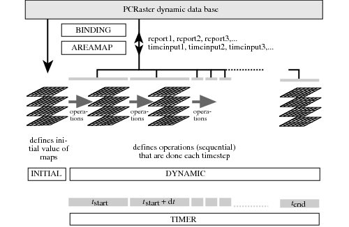
Schematic representation of a dynamic model. The areamap section defines the model area and modelling resolution. A clone map specifies the geographical location attributes of the maps used throughout the program. All maps used or generated by the model have the location attributes of the clone map in the areamap section.
The timer section controls the time dimension of the model. It specifies the duration of a model run by setting the time at the start (t(start)) and end (t(end)) of a model run. Additionally it specifies the time slice (dt) of the timestep. The number of timesteps of the model is the duration of the model run divided by the timeslice.
Spatial (maps) or non spatial attribute values at the start of the model run are given in the initial section. These values may be defined by one or more pcrcalc operations. The initial section can be seen as a static Cartographic Modelling script which sets the initial attribute values used at the start of the dynamic section, for the iteration at the first timestep.
For each timestep i, the dynamic section defines the operations that result in the (map) values for timestep i. It is an iterative section that is repeated each timestep. The dynamic section consists of one or more pcrcalc operations that are performed sequentially each timestep. At the first timestep (i = 1), the dynamic section is run using the results from the initial section. The values that result from running the dynamic section at the first timestep are called the (map) values at timestep 1. The second timestep is run, starting with the results of timestep 1. These values are used for running the dynamic section at the third timestep (i = 3), etc. Thus, the operations performed during a timestep act upon the expressions that result from running the dynamic section at the previous timestep or upon an expression value that is the same for each timestep.
Timeinput: retrieving dynamic data from the database
For each timestep, timeinput assigns a new set of map values to an expression that is used in the dynamic section. Timeinput allows the import of specified data to the dynamic section at each timestep, irrespective of the results of the previous timestep: it defines an expression that is assigned a different set of cell values for each timestep. Each timestep, timeinput queries the database for a set of cell values especially meant for that timestep and assigns these to the expression.
Timeinput is done with a timeinput pcrcalc operation in the script. This is described in Operators for timeinput.
Reporting: storing dynamic data in the database
Reporting means storing model results in the PCRaster database. Both the results of an operation in the initial or in the dynamic section can be stored in the PCRaster database. If results of the dynamic section are reported, the results are stored in the database for each timestep. This can be done in two ways. First, the result of a pcrcalc operation can be stored in the database as a set of maps, where each map gives the values for a different timestep. Second, a time series can be used to report results: each timestep, the cell values of a given set of cells are written to a time series file.
Reporting of results is done with the report keyword. The use of this keyword in the script is given in report keyword; and the timeoutput operator.
The script
Introduction, layout of the script
This The script describes the structure of a Dynamic Modelling script and its contents. The script is an ordinary ascii text file; an example was given in a Table in the beginning of this chapter. A script consists of separate sections, each with a defined function in the model. A dynamic model script contains the sections binding, areamap, timer, initial and dynamic; in this order. Each section starts with the section keyword of the section. The section keyword is followed by one or more statements that give the content of the section. Each statement is terminated by a semicolon (;) sign.
In principle, white space characters (spaces, empty lines) can be used anywhere in the script: all white space characters are ignored during execution of the script. For a structured script, we advise users to type the section keywords and the statements on separate lines. Remarks about the contents of the script are typed after a # character: everything typed on a line after this character is ignored and has no effect on the function of the model.
A statement in a section may contain keywords, names of variables, or numbers. Keywords are defined by the PCRaster Dynamic Modelling language and have a special meaning in the language. For instance the section keyword defines the start of a section in the script. Other keywords in a script are the PCRaster operators and for instance the report keyword. Keywords must always be typed in lowercase characters. Unlike a keyword, the name of a variable is chosen by the user. It may be the name of a PCRaster expression (a map or a non spatial value) or the name of a table or time series. To distinguish between keywords and names of variables, we strongly recommend that the name of a variable always begins with an uppercase character.
Binding section
In principle, if a variable is not mentioned in the binding section, the variable name in the script is directly linked to the corresponding file name in the PCRaster database: the file in the database that is used or generated during a model run has a corresponding name in the script and in the database. The binding section, identified by the section keyword binding, allows one to use a name for a variable in the script that is different from the file name of that variable in the database. This is because you probably may want to run a program a number of times, each time with a different set of data files and with a different set of resulting files. In most cases, these data files are used a large number of times throughout the program. Using the binding, you need only fill in the names of the files you want to use as input names and output names for the model run in the binding section, without changing all the file names in the rest of the program. Both file names used as input files for the model and names that are stored in the database during a model run with the report keyword may be given in the binding section.
In the binding section, the name of a file in the database is bound (linked) to its name in the model with the following statement:
- NameInModel = DatabaseFilename;
- where DatabaseFilename is the file name under which the variable is available in the database or will be stored to the database and NameInModel is the name used for the variable throughout the script.
Alternatively, a constant value can be assigned to a variable with the statement. This applies only if ModelName is a PCRaster map which is input to the model:
- NameInModel = value;
- where value is a number; NameInModel has this value throughout the program: its value cannot be changed in one of the other sections. It has no data type attached to it. Attaching a data type to the PCRaster map NameInModel with a constant value can be done using one of the data type assignment operators (boolean, nominal, ordinal, scalar, directional, ldd). An example which assigns a nominal data type to ClassMap is:
ClassMap = nominal(3);
The data type assignment operators are the only operations that can be given in the binding section, other operators cannot be used.
Not all variable names need to be mentioned in the binding; as above said, the filenames of the variables in the database can also be used directly in the script. If no variable names are bound at all, the section may be omitted from the model script.
Areamap section
The section keyword areamap defines the areamap section. It contains one statement: the name of a map which is used as clone map in the model, followed by a semi colon. This map may contain any kind of data; only its location attributes are of importance. All maps that are generated during a model run have the location attributes of the clone map. Also, all maps that are used as input to the model must have location attributes which correspond with the map in the areamap section.
Timer section
The timer section, identified by the section keyword timer, gives the time dimension of the model. It contains one statement, consisting of either three values: starttime, endtime, timeslice, e.g.
timer 1 30 1;
Or it identifies an input timeseries file, where the number of available timeseps in the timeseries defines endtime, while starttime and timeslice are set to 1:
timer rain.tss;
The iterative part of the model is run between the starttime and the endtime. The timeslice defines the time between the consecutive timesteps.
This version of the Dynamic Modelling module of PCRaster imposes restrictions on the time dimension of a model. The timeslice cannot be chosen by the user and must always be 1. Normally only the endtime is chosen, it must be a whole number larger than 1.
A starttime larger than 1 is possible but with the following consequences:
- No modifications to the initial or dynamic section are needed, assuming that the initial section puts the model in the correct state for starttime, where the dynamic section starts. All timeinput actions in the dynamic section start with reading timestep starttime.
- Output mapstacks will only be created for starttime to endtime.
- Presence of input mapstacks will only be checked for starttime to endtime
- Input timeseries files will only be read for row starttime to endtime, but must still start at 1.
- Timeoutput timeseries, will have a MV (1e31) in the rows 1 to starttime-1 except if the option —-noheader is specified.
Initial section
The initial section, identified by the section keyword initial, is meant to prepare the set of input variables which are needed to run the dynamic section at timestep 1, the first time that the dynamic section is run.
The initial section can be compared with a Cartographic Modelling script. It contains a set of pcrcalc operations which are performed consecutively, from top to bottom in the section. Each line contains a pcrcalc operation and is concluded with a semi colon (;) sign. The resulting variables of the initial section are the initial values that are used as input variables for running the dynamic section at timestep 1.
It may be that initial variables (maps for instance) for running the dynamic section at timestep 1 are already present in the PCRaster database. These do not need to be generated or changed in the initial section and can directly be used in the dynamic section, because they already have the correct value. On the other hand, all variables that are needed as input for running the dynamic section for the first time must either be defined in the initial section or must be already present in the database. This holds also for variables that have an initial value 0.
If the initial section is not needed to define the initial values of the variables it can be omitted from the script.
Dynamic section
The dynamic section, identified by the section keyword dynamic, contains pcrcalc operations that are performed at each timestep i. The operations are sequentially performed from top to bottom in the section. Each line gives a pcrcalc operation and is concluded with a semicolon (;) sign. At the start of running the dynamic at timestep i, variables have the value that results from running the dynamic at timestep i - 1. These values are used as input values for running the dynamic at timestep i. The values of the variables at the end of running the dynamic section at timestep i are the input values for running the dynamic section at timestep i + 1.
Timeinput and report in the script, running a script
Introduction
This Timeinput and report in the script, running a script describes the contents of a script meant for timeinput of data (Operators for timeinput) and reporting results ( report keyword; and the timeoutput operator). The last section (Running a script) describes how a script is run.
Operators for timeinput
Two PCRaster operators perform a timeinput operation: timeinput and timeinput... (e.g. timeinputboolean, timeinputnominal, etc.). These operations are used only in the dynamic section. Like the other PCRaster operators, the timeinput operators result in either a spatial or a non spatial expression. For each timestep, timeinput assigns specified cell values to the resulting expression, independent of the cell values at the previous timestep. The assignment of a different set of cell values to the expression for each timestep can be done in two ways:
The timeinput operator uses a set of maps in the database: the database must contain a PCRaster map with a file name extension referring to the timestep for which it is meant. The timeinput operator assigns to the expression in the dynamic section each timestep the map in the database with the extension referring to that timestep.
The timeinput... operators (timeinputboolean, timeinputnominal, timeinputordinal, timeinputscalar, timeinputdirectional and timeinputldd) use a time series. The time series is linked to a given expression with unique identifier cell values. For each timestep, the time series gives cell values for these unique identifiers. These cell values are assigned to the timeinput expression in the dynamic section on basis of the unique identifiers on the unique identifier expression.
For a detailed description of the timeinput operations, see timeinput and timeinput.... Time series format gives the format of time series.
report keyword; and the timeoutput operator
- The report keyword stores the result (which is always on the left hand side) of a pcrcalc operation to the database. Reporting is done by typing the keyword report before a pcrcalc operation: report VariableName = operation;
- for instance:
report NOStdDev = sqrt(NOVariance);
has the effect that the result (NOStdDev) of the pcrcalc operation is stored to the database. In a script, a VariableName cannot be used for report more than once.
The report keyword has no effect on the pcrcalc operation that is done, the only effect of report is that it stores the result of the operation in addition to computing it. If results of the iterative dynamic section are reported, the results are stored in the database for each timestep. The model results for each timestep can be reported in two different ways; the sort of report that is made depends on the sort of operation that is prefaced with the report keyword.
First, the results of an ordinary pcrcalc operation can be reported. If the result of the operation preceded with the report keyword is a map, each timestep the whole map is stored in the database with a filename that refers to the timestep under consideration. The file names of these maps in the database consist of two parts: the suffix and an extension. The suffix corresponds to the name of the variable that is prefaced by the report keyword. The suffix is followed by the time extension which corresponds with the time of the timestep at which the map is generated. The filename has a format that corresponds with the historic MS-DOS rules for filenames: 8 characters, a dot and 3 characters. This is best illustrated by an example. Imagine a model with starttime = 1, endtime = 1200. In the dynamic section, the statement
report Snow = Snowfall * 2;
stores 1200 maps in the database with filenames Snow0000.001, Snow0000.002,...Snow0001.199, Snow0001.200. If this statement were put in the initial section only one map is stored in the database with filename Snow. Remember that it is not possible to report variable name Snow more than once: both in the initial and in the dynamic section.
Maps stored in the database with the report keyword have the filename format which is also needed for the timeinput operation.
If the result of the pcrcalc operation which is reported is a non spatial value it is automatically stored as a time series. At the end of the model run, the time series will contain the resulting non spatial value for each timestep.
The second way in which a report can be made is reporting results of a pcrcalc operation especially meant for reporting: the timeoutput operator. This operators always create a time series and must always be prefaced with the report keyword. They are only used in the iterative dynamic section. The timeoutput operator reports cell values of a specified cell or cells of an expression to a time series in the database. The result of one map operation resulting in a non spatial value is always written to a time series. It is meant to report statistics of a map for each timestep. Time series format gives the format of time series.
Running a script
A Dynamic Modelling script is run in PCRaster by typing:
- pcrcalc -f NameOfModel
- where NameOfModel is the file name of the ascii formatted model script.
How to make a dynamic model
The soil moisture model with evapotranspiration
This following sections give some examples of a Dynamic Modelling script. We describe how the change in soil moisture content as a result of precipitation and evapotranspiration can be modelled using the PCRaster Dynamic Modelling language. In this section, we start with a script for a simplified model, without rain during a model run. The next section (Soil moisture model with timeinput: rain) describes a somewhat more complicated model, incorporating rain modelled with a timeinput operation.
Evapotranspiration is the combined water loss to the atmosphere by evaporation from the soil and transpiration from plants. The actual evapotranspiration Eact (mm/day) from a crop can be calculated with the relation (chow88): Eact = ks x kx Eref (1) where Eref (mm/day) is the reference crop evapotranspiration of a specified green grass surface with a soil not short of water. Eref depends on the weather conditions during the day; for the sake of simplicity it is assumed to be constant. The soil coefficient ks (0 =< ks =< 1) mainly depends on the soil water content of the soil and is also assumed to be one: the soil is not short of water. The crop coefficient kc depends on the sort of crop and may have a value of 0.2 for almost bare ground up to 1.3 for vegetation that transpires at a great rate, such as corn. It is assumed that a map is available with the crop coefficient values, recoded from a land use map. So, the model assumes a temporarily constant evapotranspiration which for each day is given by: Eact = kc x Eref (mm/day) (2)
As a result of evapotranspiration the soil moisture content (mm) decreases. For simplicity, it is assumed here that evapotranspiration is the only flow that changes the soil moisture content. No other flows, such as infiltrating rain or percolation to the deeper groundwater occur. The figure below gives the change with time, with a timestep of 1 day, in the soil moisture content at a gridcell according to this concept. This figure also shows the critical moisture content which is the moisture content value below which shortage in soil moisture may occur.
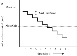
Change of Soil moisture content (mm) with time, timestep one day. Included process: evapotranspiration. MoistInit: moisture content at start of model run (mm); MoistCrit: critical moisture content (mm); Eact: actual evapotranspiration (mm/day).
Now let’s make a model for the process described above and shown in the Change of Soil moisture content (mm) with time, timestep one day. Included process: evapotranspiration. MoistInit: moisture content at start of model run (mm); MoistCrit: critical moisture content (mm); Eact: actual evapotranspiration (mm/day).. Inputs for such a model are maps containing for each cell the initial moisture content and the critical moisture content. Additionally, in order to calculate the actual evapotranspiration a map with the crop coefficients for each cell and one constant value of the reference crop evapotranspiration is needed. The model must calculate (with equation (2)) and store in the database for each timestep a map with the moisture content at that timestep. Here we also assume that the model builder wants to know for each timestep the maximum moisture content in the study area and the area of land that has a moisture content below the critical value. Table 2 (below) gives the script for such a model. Two maps already present in the database are bound to the model names MoistMeas and Kc. Respectively, these are Moist952.map which contains measured moisture contents, which may be based upon an interpolation of field measurements, and CrCoef95.map which contains the crop coefficient value for each cell. The MoistCrit is the critical moisture content which is assumed to have a constant value of 20 mm over the study area. The reference crop evapotranspiration (modelname Eref) has a constant value of 8 mm/day. The binding also gives the file name under which the output time series TimeSeriesMin and TimeSeriesMax (defined in the dynamic section) is stored to the database.
Dynamic modelling script for change in soil moisture content; included process evapotranspiration.
# model for calculation of reduction in soil moisture content
# incorporated processes: evapotranspiration
# timestep one day

binding
 MoistMeas = Moist952.map;   # measured moisture content (mm)
 MoistCrit = scalar(20);     # critical moisture content (mm)
 Eref = scalar(8);           # reference crop evapotranspiration (ETPrc)
                             # mm/day
 Kc = CrCoef95.map;          # crop coefficient map
 TimeSeriesMax = Max8.tss;   # time series binding
 TimeSeriesMin = Min8.tss;   # time series binding

areamap
 Clone.map;                  # clone map with location attributes of maps
                             # used in model

timer
 1 30 1;                     # starttime: 1 (first day)
                             # endtime: 30 (thirtiest day)
                             # timeslice 1 day
                             # as a result 30 timesteps (iterations)

initial
 report Eact = Kc * Eref;    # actual evapotranspiration (mm)
 Moist = MoistMeas;          # initial moisture content is measured
                             # moisture content (mm)

dynamic
 report Moist = Moist - Eact;               # moisture content (mm)
 MoistBelowCrit = Moist le MoistCrit;       # results in boolean map
 report TimeSeriesMax = mapmaximum(Moist);
 report TimeSeriesMin = mapminimum(Moist);
                                            # reports to a time series
All maps used in the model must have the same location attributes. The areamap section defines a map with these location attributes. Here it is the map Clone.map, available under that name in the PCRaster database.
The timer sets the model time. The model starts at time = 1 and ends at time = 30, with a timestep of 1. As a result it consists of 30 timesteps which represent 30 days of evapotranspiration. The starttime is 1, so the results of running the dynamic section for the first time, at the first timestep, are stored with time extension 1.
The initial section defines the initial moisture contents at the start of the model run: these are assumed to be the measured moisture contents stored in the map MoistMeas. The actual evapotranspiration according to equation (2) is also defined. It does not change during the model run, for this reason it has been put in the initial section. It is also reported: the initial moisture content is stored to the database under the name Moist.
The dynamic section contains three pcrcalc operations. For each timestep, first the moisture content for that timestep is calculated, by subtracting the actual evapotranspiration from the moisture content of the previous timestep. For each timestep, the report keyword provides that the moisture content is stored to the database. At the end of the model run, the database will contain 30 moisture content maps. These have filename extensions referring to the time of the timestep at which each map has been generated. The resulting map of the first timestep at time = 1 is stored under the name Moist000.001, the map of the second timestep at time is 2 is stored as Moist000.002 etc. Remember that it would not be possible to report also the operation Moist = MoistMeas; in the initial section. That would result in a report of Moist which is made two times in one model which is not allowed.
MoistBelowCrit is calculated in the second statement using the value for Moist that results from the pcrcalc operation in the first statement. MoistBelowCrit is a Boolean map that contains a Boolean TRUE (cell value 1) for cells that have a moisture content equal to or below the MoistCrit value and a Boolean FALSE for cells that still have a moisture content larger than MoistCrit.
The third statement reports a timeseries with model name TimeSeriesMax. Each timestep, the maximum cell value of the map Moist is written to the time series. The binding section defines that the table is stored under the file name Max8.tss. This is neatly done: for a next run with a slightly changed model (for instance with a Eact value of 6), the user only needs to bind the TimeSeriesMax to a new filename, for instance Max6.tss. In this way, it is relatively simple to run different scenarios, each time only changing the values and filenames in the binding.
Soil moisture model with timeinput: rain
Now, we build on the model given in the previous section by adding rain to the soil during the 30 days of evapotranspiration. We assume that all rain water immediately infiltrates in the soil. If the saturated soil moisture content is reached as a result of rain water infiltration, the remaining rain water is not added to the soil moisture anymore. This excess in rain will run off. Here, the runoff process is not incorporated in the model: it is assumed that the saturated moisture content is not exceeded as a result of infiltrating rain. The evapotranspiration rate is assumed not to be influenced by the infiltrating rain water. So no changes are made in the model with respect to evapotranspiration. The figure below shows the temporal change in soil moisture content as a result of evapotranspiration and infiltrating rain.
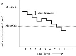
Change of Soil moisture content (mm) with time, timestep one day. Included process: evapotranspiration and rain. MoistInit: moisture content at start of model run (mm); MoistCrit: critical moisture content (mm); Eact: actual evapotranspiration (mm/day). Rain falls at time = 6 and 7 days.
The model example below gives the sequential modelling script for evapotranspiration and infiltration. The binding section gives the model names for respectively the saturated soil moisture content map and the time series with the rain in millimetres for each timestep. The table below gives the ascii formatted time series file Rain.tss that is used. Dynamic modelling script. Included processes: evapotranspiration and infiltrating rain.
# model for calculation of reduction in soil moisture content
# incorporated processes: evapotranspiration and infiltration of rain
# timestep one day

binding
 MoistMeas = Moist952.map;   # measured moisture content (mm)
 MoistCrit = scalar(20);     # critical moisture content (mm)
 Eref = scalar(8);           # reference crop evapotranspiration;
                             # (ETPrc) mm/day
 Kc = CrCoef95.map;          # crop coefficient map
 TimeSeriesMax = Max8.tss;   # time series binding
 TimeSeriesMin = Min8.tss;   # time series binding
 RainTimeSeries = Rain.tss;  # timeseries with amount of rain at each
                             # timestep (mm/day)

areamap
 Clone.map;                  # clone map with location attributes of maps
                             # used in model

timer
 1 30 1;                     # starttime: 1 (first day)
                             # endtime: 30 (thirtiest day)
                             # timeslice 1 day; as a result
                             # 30 timesteps (iterations)

initial
 report Eact = Kc * Eref;    # actual evapotranspiration (mm)
 Moist = MoistMeas;          # initial moisture content is measured
                             # moisture content (mm)

dynamic
 Rain = timeinputscalar(RainTimeSeries, 1);
 report Moist = Moist + Rain - Eact;  # moisture content (mm)
 MoistBelowCrit = Moist le MoistCrit; # results in boolean map

 # reports to a time series
 report TimeSeriesMax = mapmaximum(Moist);
 report TimeSeriesMin = mapminimum(Moist);
In the first statement of the dynamic section, the timeinputscalar operator reads the RainTimeSeries and assigns each timestep the amount of rain to Rain. In the second statement, Rain is added to the soil moisture Moist.
The remaining statements give the operations for the evapotranspiration process and the report. These have not been changed compared to the model given in the previous section.
Time series Rain.tss: rain at the study site.
Rain, 1-30 July 1995
2
time
rain (mm)
1      0.0
2      0.0
3      5.2
4      0.0
5      23.1
6      40.1
.
.
- lines for 7 to 28 not shown -
.
.
29     0.0
30     0.0