The Database

Introduction

This chapter describes the database of the PCRaster package. After a general introduction with the concepts behind the structure and the components of the database (Concepts, kinds of data used in the database), the components of the database wll be described in further detail, with emphasis on the practical on the practical aspects (formats, data types for instance. First the structure of PCRaster maps, like location attributes, missing values and data types will be described (PCRaster maps) after which the different types of formats of tables, time series and point data column files will be explained (Table format, Time series format and Point data column file format). Of these sections, you will need the time series part (Time series format) only if you want to use the module for Dynamic Modelling (see Dynamic modelling). How to manage the database (data import, export, conversions etc.) and how to perform other GIS functions is described in How to Import or Export Data, Display Maps, Global Options.

Concepts, kinds of data used in the database

Four kinds of data are used in the PCRaster database. Data from 2D areas are represented by raster maps. These PCRaster maps have a special PCRaster format that enables simple and structured manipulation of spatial data in the package. It is the most important kind of data in the database: almost any PCRaster operation uses and/or generates a PCRaster map. For analysis of PCRaster maps with other software packages, conversion to ascii format is needed. The remaining three kinds of data (tables, time series and point data column files) represent relations between PCRaster maps, temporal data and data from points respectively. These kinds of data are in ascii format; as a result these can also be analysed with other software packages, without conversion.

In PCRaster a stack of PCRaster map layers represents the landscape, where each map layer represents one attribute, see A stack of PCRaster maps resulting in a 2.5 D representation of the landscape. One cell is shown; its property is defined by the attribute values stored in map layers Map1, Map2, Map3,.... The discretization of the spatial domain results in cells. At each cell location, the total information for that cell is represented by the values of the different layers at that cell. The representation described here is sometimes referred to as 2.5 D: the lateral directions are represented in real, while a certain kind of vertical dimension is implemented using several layers.

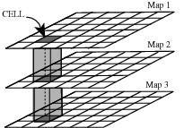
A stack of PCRaster maps resulting in a 2.5 D representation of the landscape. One cell is shown; its property is defined by the attribute values stored in map layers Map1, Map2, Map3,...

The spatial characteristics of a PCRaster map are defined by its geographical location attributes . These define the shape and the area covered by the map and the size of the cells.

The kind of attribute represented by the layers controls the type of operations that can be done with the data stored in the layer. This knowledge is implemented in the PCRaster package by the idea of data types: each PCRaster map layer has a data type attached to it. Six data types are recognized. Data types for data in classes are the boolean, nominal and ordinal data types. The boolean data type is meant for data that may only have two values: TRUE or FALSE. Boolean logic can be applied to maps of this data type. The nominal data type represents data with an unlimited number of classes, for instance soil groups. The ordinal data type also represents data in classes; unlike the nominal data type it includes the concept of order between the classes, for instance classes that represent income groups. The scalar and directional data type represent continuous data ; the scalar data type for data on a linear scale, for instance elevation, the directional data type for data on a circular scale, for instance aspect in the terrain. The ldd data type represents a map with a local drain direction network. For each cell, a local drain direction map contains a pointer to the neighbouring cell to which material (for instance water) will flow to. The direction of these pointers is represented by ldd codes.

PCRaster maps describes the format of maps, including the location attributes, data types and legends in detail.

Relations between PCRaster maps can be defined by tables, which is the second kind of data used in PCRaster, see A table defining relations between PCRaster map layers; using these conditions a NewMap is generated, on a cell by cell basis. In a table, map layers are combined by specifying keys. Each key gives a certain combination of cell values of the map layers 1,2,3,... A key may be for instance: the cell of map 1 must have a value 6, the cell of map 2 a value larger than 200 and the cell of map 3 must contain a negative value. Using the keys in a table a new map layer can be generated which contains information taken from several layers. For instance a soil map, vegetation map and a slope map can be combined using keys in a table containing the classes of these maps, generating a new map with landscape classes. Also a table can be used for determining the number of cells that match the conditions given in the keys. Table format describes the format of tables.

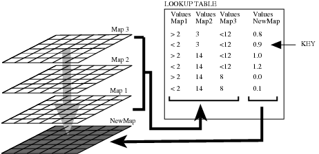
A table defining relations between PCRaster map layers; using these conditions a NewMap is generated, on a cell by cell basis

The third kind of data used in PCRaster is the time series. In Dynamic Modelling, time series are linked to a PCRaster map to control spatial data that vary over time and space: for each time step, a different spatial data set that represents a certain variable used in the model can be imported or stored. For instance when simulating evapotranspiration of water in a catchment, for each time step the amount and the spatial distribution of rain water can be given in a time series; the amount of water that evaporates from a certain part of the map can be stored in a different time series. The time series is a table that crosses the unique identifier values on a PCRaster map with the numbers of the successive time steps used in the model. During a model run, it is read from top to bottom. If the time series is used for data input to the model, each unique identifier value on the PCRaster map is assigned the value linked to that unique identifier in the time series. This is done for each time step. If the time series is used to store data, for each time step the model results for certain areas specified on the PCRaster map can be assigned to the time series. Time series format describes the format of time series.

In addition to spatial data in raster format, point data are used in the PCRaster package, stored as point data column files, the fourth sort of data used. Point data consist of a x,y coordinate and one or more attribute values. Quite often data will be available in this format, especially if they are gathered through field study. In the gstat module point data column files can be used for analysis of spatial structures with the variogram tools and for interpolation to a raster (in PCRaster map format) of estimated values using (block) kriging. Point data column file format describes the format of point data column files.

PCRaster maps

Introduction

This section describes the format of the main sort of data used in the PCRaster package: the PCRaster map, which contains spatial data in raster format. A header is attached to each PCRaster map; it contains both the location attributes and the data type of the map. The location attributes define the position of the map with respect to a real world coordinate system, the size and shape of the map and its resolution (cell size). The sort of attribute stored in the map is given by the data type of the map. The data type determines the PCRaster operations that can be performed on the map. Data typing used in PCRaster helps to structure your data.

If you start a project, and want to import data to the PCRaster package in PCRaster map format it is wise first to make a map containing the header with the correct location attributes and the data type of the first data set you want to import. How this is done is described in PCRaster maps: database management. This section also describes other aspects of database management with a map.

Location attributes, missing values

This section gives an overview of the geographical location attributes linked to a PCRaster map.

The location attributes projection, xUL,yUL, cell length, number of rows, number of columns and angle are used to define the position of the map with respect to a real world coordinate system and the shape and resolution of the map. The figure below shows schematically a PCRaster map of a study area and the location attributes used. As shown, the location attributes define the map with respect to the real world coordinate system (an ordinary x,y coordinate system).

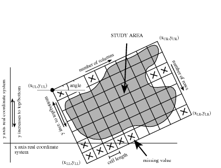
Location attributes used to define the spatial characteristics of a PCRaster map.

The choice of the location attributes must be based upon the shape of the study area and the data set you want to store in the map. PCRaster maps always have a rectangular shape, but the shape and size of the map does not need to correspond exactly with the shape of the area studied, as shown in the figure above: during data import to the PCRaster map the cells in the map outside the study area are assigned missing values. A missing valued cell is a cell which contains no attribute value. Missing valued cells are considered not to be included in the study area: PCRaster GIS and Cartographic or Dynamic Modelling operators ignore the missing valued cells. In general, cells that have a missing value on an input map of an operation are assigned a missing value on the resulting output map(s) also.

For a complete description of the choice of the location attributes related to the data set that will be stored in the map, see Creation of a PCRaster map; data import.

The location attributes have the following meaning; see also Location attributes used to define the spatial characteristics of a PCRaster map.:

projection

The projection of the real coordinate system which will also be assignednto the PCRaster map, is assumed to be a simple x,y field (also used innbasic mathematics). The x coordinates increase from left to right. The yncoordinates increase from top to bottom or from bottom to top. This cannbe chosen; from top to bottom is default.

xUL,yUL

The xUL, yUL are the real world coordinates of the upper left corner of the PCRaster map. The location of the PCRaster map with respect to the real world coordinate system is given by this corner: if a rotated map is used (an angle not equal to zero), it is rotated around this point (so rotation over 90 degrees will result in a xUL, yUL that is at the bottom left side in Location attributes used to define the spatial characteristics of a PCRaster map.). Other PCRaster map corners are xLL, yLL ; xUR, yUR ; xLR , yLR .

cell length

The cell length is the length of the cells in horizontal and vertical direction.nThis implies that cells in a PCRaster map are all of the same size andnalways square. The cell length is measured in the distance unit of the realnworld coordinate system.

number of rows, number of columns

The number of rows and the number of columns are the number of rows andncolumns of the PCRaster map respectively. The cell length multiplied bynthe number of rows and number of columns is the height and width of thenPCRaster map, respectively (in distance units of the real worldncoordinate system).

angle

The angle is the angle between the horizontal direction on the PCRasternmap and the x axis of the real world coordinate system. It must benbetween -90 and 90 degrees; a map with a positive angle has been rotatedncounter clockwise with respect to the real coordinate system, a map withna negative angle has been rotated clockwise. In most cases an unrotatednmap will be sufficient (angle = 0 degrees), see also Creation of a PCRaster map; data import.

Data types

Introduction

Data stored in PCRaster maps can be grouped according to the sort of attribute they represent. For instance, a distinction is often made between attributes that are stored in maps as classified data (for instance soil classes) or continuous data (for instance elevation). In PCRaster, attribute information is linked to each map by specifying one of six data types. Each data type imposes a distinct domain of values that may occur on a map (whole values or fractional values, range of possible values) and whether some kind of order/scale is represented by the data (with or without order; linear or directional scale). If a legend is attached to a map, the map is subtyped by its legend: the attribute stored in the map is not only specified by the data type of the map, but also by the legend. Also the domain of a subtyped map is determined by the legend: it consists only of the map values linked to the classes given in the legend. As a result, PCRaster prevents some operations that otherwise would combine maps with different legends. For instance a landuse map and a soil map cannot be joined laterally together. The legend of a map and the resulting subtype is described in Legends.

The data type mechanism used in PCRaster will help you understand and organize your ideas about the attributes stored in your database or used in some kind of spatial model. The data types will prevent you from doing operations that are nonsense: each time a operation is done, the system checks the data type of the input maps and if the operations would result in nonsense an error message is given. Also, for some PCRaster operators the system adapts the way the operation is done to the data type of the input maps (this is called polymorphic behaviour of GIS operators). Additionally, the map resulting from an operation is given the data type that fits the sort of data that result from the operation.

or double real or large integer for scalar and directional data and small integer Most data types have a distinct cell representation . The cell representation is not related to the concept of data type checking in the GIS, and for ordinary use it is of little importance: it only determines the way the values of the cells are stored and processed in the computer. The cell representations used in PCRaster are single real for nominal and ordinal data. These are represented in the computer by REAL4 (single real), REAL8 (double real), UINT1 (small integer) and INT4 (large integer). UINT1, REAL4, REAL8, UINT1 and INT4 are also applied in other software, see for an exact description a standard book about computers in your library. By default, PCRaster automatically chooses the cell representation for each data type, so for ordinary use you do not need to take care of the cell representation. In some cases, especially if you want to store extremely large or small data values at a high precision you may want to choose a cell representation another than the default. This can be done with global options for defining cell representations. The cell representations for each data type are given in the next sections.

Maps (and nonspatials)

List of data types, domaines for default cell representation, without legends

data type	description attributes	domain	example
boolean	boolean	0 (false), 1 (true)	suitable/unsuitable, visible/non visible
nominal	classified, no order	-231 ... 231, whole values	soil classes, administrative regions
ordinal	classified, order	-231 ... 231, whole values	succession stages, income groups
scalar	continuous, lineair	-1037...1037, real values	elevation, temperature
directional	continuous, directional	0 to 2 pi (radians), or to 360 (degrees), and -1 (no direction), real values	aspect
ldd	local drain direction to neighbour cell	1...9 (codes of drain directions)	drainage networks, wind directions

Boolean data type

The domain of the Boolean data type is 1 (Boolean TRUE) and 0 (Boolean FALSE). It is used for all attributes that only may have a value TRUE or FALSE, for instance ‘suitable or unsuitable for maize’, or to specify cells that come into a class or do not come into a class, for instance cells with a watch-tower or cells without a watch-tower. A legend can be made for a map of data type Boolean; it has no effect on the domain of the map.

Ordinal data type

The ordinal data type is used for classified data that represent some kind of order. For instance stages of succession or soil texture measured at an ordinal scale (silt, sand, gravel for instance). Any number in the domain can be chosen to represent an ordinal class, but normally for the first class an ordinal value of 1 is chosen and for the next classes the values 2, 3,.. etc.; a value of 0 is chosen for cells that do not come into a class. If the cell representation large integer is chosen (default) the domain consists of all whole values between -2³¹ and 2³¹. If the small cell representation is used, the domain consists of whole values equal to or between 0 and 255.

A legend can be attached to a map of ordinal data type, see Legends. This results in subtyping of the map.

Nominal data type

The nominal data type is used for classified data without order. It represents attributes described by classes, for instance a map with soil classes.

Any number in the domain can be chosen to represent an ordinal class, but normally for the first class an nominal value of 1 is chosen and for the next classes the values 2, 3,.. etc.; a value of 0 is chosen for cells that do not come into a class. If the cell representation large integer is chosen (default) the domain consists of all whole values between -2³¹ and 2³¹. If the small cell representation is used, the domain consists of whole values equal to or between 0 and 255.

A legend can be attached to a map of nominal data type, see Legends. This results in subtyping of the map.

Scalar data type

The scalar data type is used for continuous data that do not represent a direction, for instance number of inhabitants, air particle concentration, amount of rain, elevation, or wind speed. The default cell representation is single real, which allows for storing and processing real values of data between -1*10³⁷ and 1*10 ³⁷, using a maximum of six decimals.

Directional data type

The directional data type is used for continuous data that represent a direction. The domain depends on the sort of directional data that is used: if the global option --degrees is set (for global options see Global options), the domain consists of real values equal to 0 or between 0 and 360 degrees and the number -1 for cells without a direction (-1 and [0,360> which means that 360 is not in the domain). If the global option --radians is set the direction is given in radians, the domain is [0,2pi> and the number -1 for cells without a direction. The value -1 is not a missing value: it represents a cell for which no direction can be given. For instance a cell in a flat terrain does not have an aspect; as a result it has the value -1 on a map with aspects. The direction in the map of a directional value 0 depends on the location attribute angle of the map, see Location attributes, missing values : a cell value of 0 points to the North of the map (the y direction of the real world coordinate system), the remaining values increase in clock wise direction. In most cases the top of the map will be the North (location attribute angle = 0 degrees). In these cases a directional value 0 is to the top of the map and 90 degrees (East) corresponds with a direction to the right side of the PCRaster map.

The directional data type can be used for all attributes that have a circular scale, for instance orientation or a year scale. Default the cell representation is single real; double real can be chosen for a higher precision, but in almost any case single real will give satisfying results. Note that statistics of directional data, like mean and variance, are computed in a different way than for scalar data (see also mardia72). So always use the directional data type for directional data: PCRaster will automatically apply statistics for directional data to the map values.

Ldd data type

The ldd data type is used for maps that represent a local drain direction network . A local drain direction network is made up of a network of cells; each cell has a whole value from 1 to 9. These codes identify the neighbour of the cell to which material flows. The values have the meaning shown in in the figure below; note that the values are chosen to resemble the numeric key pad of your computer.

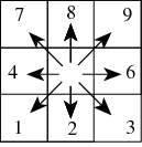
Directions of ldd codes.

A value 5 (centre) defines a cell without local drain direction (a pit). For instance, during transport of material, a cell with value 3 designates flow to the bottom right neighbouring cell. The value 5 represents a pit : this is a cell without drainage to one of its neighbours.

Since the local drain direction network on a map of ldd data type defines a relationship between cells, a map of this data type must meet some requirements to safeguard these relationships. If a map meets these requirements it contains a so called sound ldd network. A ldd map is sound if it is a map containing only whole values from 1 to 9 or missing values. Additionally the values on the map must be ordered in such a way that each downstream path starting at a non-missing value cell ends in a pit cell. A downstream path consists of the consecutively neighbouring downstream cells; the pit cell at the end of the path is called the outlet point of the cell where the path started.

Here is a (non exhaustive) list of situations which cause a ldd to be unsound:

• a cell on the border of the map has a local drain direction to the outside of the map. For example, a ldd code 7, 8 or 9 on the first (top) row of cells or a value 7, 4 or 1 on the first (left) column of cells of the map.
• a cell with a local drain direction to a cell with a missing value. For example a cell with a value 3 while its bottom right neighbour is a missing value.
• The ldd contains a cycle. A cycle is a set of cells that do not drain to a pit because they drain to each other in a closed cycle. The smallest cycle consists of two cells with local drain directions to each other; larger cycles may consist of several cells.

A ldd that is not sound cannot be used for PCRaster operations. So you must always prevent operations that may generate an unsound ldd. Normally, a ldd network is made from an elevation map using the operator lddcreate. This will always result in a ldd that is sound. Other operations that can be used to generate a map of ldd data type will almost always result in a ldd that is unsound; examples are asc2map, col2map, cover, lookup. Some operations for making changes in a ldd must be done with care: editing using aguila and also cutting in a ldd map: always use the operator lddmask for cutting instead of for instance if then, if then else. A ldd that is not sound can be made sound using the operator lddrepair. Always use this operator if you are not sure whether your ldd is sound; it will be repaired if it is unsound.

Legends

Legend labels can be attached to boolean, nominal and ordinal maps with the operator legend.

Table format

This section describes the format used for tables. The concept of tables specifying relations between PCRaster maps was discussed earlier in this chapter (Concepts, kinds of data used in the database). For creating and editing a table see Tables: database management.

Two formats for tables are used, a column table and a matrix table. By default, PCRaster uses column tables. If you want to specify relations between only two maps it is sometimes better to use matrices instead. This is done by setting the global option --matrixtable (for global options, see Global options). The formats of tables are:

column table

In the column table relations between the values of several maps expression1, expession2,...expressionN are given, where an expression can be a PCRaster map or a computation with PCRaster operators resulting in a PCRaster map. For each combination of values of expression1, expression2,...expressionN a new value can be specified.

For example:

<2,>	3	<,12>	1
<,2]	3	<,12>	3
<2,>	14	<,12>	7
<,2]	14	<,12>	9
<2,>	14	8	4
<,2]	14	8	8

The first, second and third column give the values of expression1, expression2 and expression3 respectively; the fourth column contains the value fields.

The column table is an ascii file that consists of a number of N+1 columns. The first N columns are key columns, where N is the number of maps. The key columns consist of key fields; each key field is one value or a range of values. The key fields in the first column are linked to cell values of expression1, the key fields in the second column to values on expression2, and so on, where the key fields in the nth column are linked to values on expressionn. The last column (column number n+1) contains so-called value fields; these are new values that may be assigned to a new PCRaster map. Sometimes, if the table operator is used these will contain the number of cells (score) that match the key. Each row in the column table is called a tuple. Of course, it consists of n key fields and one value field.

The fields are separated by one or more spaces or tabs. The number of spaces or tabs does not matter. A value field is one single value. A key field is a single value, or a range of values, where a range of values is typed as: ‘[‘ or ‘<’ symbol, minimum value, comma (, character), maximum value, ‘]’ or ‘>’ symbol. The minimum and maximum values are included in the range if square brackets (‘[‘ and ‘]’) are used, they are not included if point brackets (‘<’ or ‘>’) are used. Omitting a value in the range definition means infinity. Ranges can be used for nominal, ordinal, scalar and directional data types. Values in keys are typed as an ordinary number (for instance 24.453) or by using base ₁₀ exponentials (for instance 32.45e3 means 32450). Column tables may consist of as many tuples as needed. Remember that when linking maps with the operator lookup , for each cell the value field is assigned of the first tuple (from top to bottom) that matches the set of expression1, expression2,...expressionN values of the cell.

matrix table

A 2D matrix table contains the relations between two expressions expression1, expression2, where an expression is a PCRaster map or a computation with PCRaster operators resulting in a PCRaster map.

Example:

-99	1	2	3	4
12	6.5	6.5	6	6
14	-4	-4	-4	-4
16	-13	-13	-12	-12

The fields in the first row contain values of expression1; the fields in the first column contain values of expression2. The field in the top left corner is a dummy field. The remaining fields are value fields.

The matrix table is an ascii table with the following format. The first field in the top left corner of the matrix is not considered during PCRaster operations but is necessary to align the matrix; it is a dummy field and may have any value. The first row consists of this dummy field and the key fields which are linked to expression1. The first column consists of the dummy field and the key fields which are linked to expression2. The key fields may be one single value or a range of values, where a range is specified in the same way as it is done in a column table (see above). The remaining fields in the table are value fields and consist of the values which will be assigned to a new map. Or, if the table operator is used these will contain the number of cells (score) that match the key. In horizontal direction, fields must be separated by one or more spaces or tabs. All fields must be filled in.

Time series format

This section gives the format used for time series. Creating and editing a time series will be discussed later on (Creating and editing time series, as will the use of timeseries in dynamic modelling (Dynamic modelling).

The contents and the format (number of rows) of a time series must match the dynamic model for which the time series is used, especially the time dimension of the model. For a description of the time dimension and the terms used, see Timer section. Two types of format for a time series are used: the time series with a header and a plain time series without header. Both are ascii formatted text.

time series with a header

Example of a time series file with a header, giving the temperature at three weather stations, meant for input or the output of a model with starttime 1, endtime 8 and timeslice 1.

Temp., three stations
4
time
station 1
station 2
station 3
1  23.6  28  23.9
2  23.7  22  24.8
3  23.7  22  25.8
4  21.0  24  21.1
5  19.0  24  17.2
6  18.9  22  17.9
7  16.2  22  15.9
8  16.8  24  14.9

A timeseries file with a header has the following format:

line 1: header, description

line 2: header, number of columns in the file

line 3: header, time column description

line 4 up to and including line n + 3: header, the names of the n identifiers to which the second and following columns in the time series are linked.

subsequent lines: data formatted in rows and columns, where columns are separated by one or more spaces or tabs.

Each row represents one timestep I at time t(I) in the model for which the time series is used or from which the time series is a report; the first row contains data for timestep I = 1, the second row for timestep I =2, etc. The first column contains the time t at the timesteps. At the first row which contains data for the first time step (I = 1) it is always the starttime t(1). For the following consecutive rows, the time in the first column increments each row with the timeslice dt of the model: in the Ith row (Ith timestep) the time is t(1) + (I-1) x dt. The remaining columns (column number 2 up to and including number N+1) contain values related to the N identifiers, where column number I is linked to the unique identifier value I-1. So, the second column contains values related to a unique identifier of 1, the third column contains values related to a unique identifier of 2 etc.

plain time series

This is a file formatted like the time series file with header, but without the header lines.

Point data column file format

This section gives the format used for point data column files. The creation of a point data column file and the conversion between point data column files and PCRaster maps will be discussed in the next chapter (Point data column files: database management).

Ascii formatted column files are used for representation of point data in PCRaster. A column file consists of two columns containing the x and y coordinates respectively and one or more columns containing data values. Two types of column files can be used in PCRaster: a column file in simplified Geo-EAS format or a plain column file

column file in simplified Geo-EAS format

Example of a column file in simplified Geo-EAS format:

pH data January 17
4
xcoor
ycoor
pHfield
pHlab
349.34  105.03  3.4  4.1
349.36  102.51  3.4  4.1
348.89  104.00  3.6  4.1
348.44  102.68  3.5  4.1
349.89  104.72  3.8  4.1

It has the following format:

line 1: header, description

line 2: header, number (n) of columns in the file

line 3 up to and including line n + 2: header, the names of the n variables

subsequent lines: data which are formatted in at least three columns containing the x coordinates, y coordinates and values, respectively. Each line contains a record. The separator between the columns may be one or more whitespace character(s) (spaces, tabs) or ascii character(s).

plain column file

This is a file formatted like the simplified Geo-EAS format, but without header lines. The column separator may be chosen by the user. Fields with the x coordinates, y coordinates and values in the columnfile may contain the characters: -eE.0123456789. Fields may not be empty, valid fields are for instance: 25.11, -3324.4E-12 (which represents -3324.4 x 10-12), .22 (which represents 0.22).