Cartographic Modelling
Introduction
This section describes the Cartographic Modelling part of the PCRaster package. As noted in GIS and Cartographic Modelling this module includes both analysis of maps using PCRaster operators for Map Algebra from the command line and using PCRaster operators for Cartographic Modelling. In Cartographic Modelling, PCRaster operators are used to build static models by combining several operations into script files. Using these script files, you can let the computer perform several PCRaster operations consecutively and automatically.
Cartographic Modelling does not include a concept of time: the operations that are performed represent one static change in the property of the cells. If you want to make models that incorporate processes over time (for instance hydrologic models using time series) you have to use the Dynamic Modelling module, which is described in Dynamic modelling. This module uses the same operators as used in Cartographic Modelling, but they are combined in a different way.
The first section of Cartographic Modelling describes the general approach to operations for Cartographic Modelling ( General approach to Cartographic Modelling). The subsequent sections describe the four classes of Cartographic Modelling operations: point operations (Point operations), neighbourhood operations (Neighbourhood operations), area operations ( Area operations) and map operations (Map operations). For an exhaustive list of all PCRaster operators included in these functional classes see Functional list of applications and operations. Command syntax and script files for cartographic modelling describes the general rules for instructing your computer to perform PCRaster operations for Map Algebra and Cartographic Modelling (command syntax and script files).
If you have operated a geographical information system before and you have knowledge of Map Algebra, you may want to skip General approach to Cartographic Modelling up to and including Map operations and use Functional list of applications and operations to get an overview of the operators. You should always read Command syntax and script files for cartographic modelling, because it contains important practical information.
General approach to Cartographic Modelling
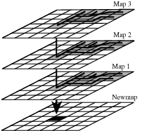
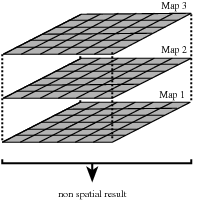
In PCRaster, a stack of map layers represents the landscape. Each map layer Map1, Map2, Map3,... can be thought of as defining an attribute, containing geographical data for that attribute. The property of each cell is defined as consisting of the set of attribute values stored to that cell on the map layers.
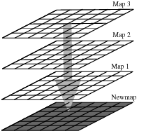
Generation of a NewMap as a result of maplayers Map1, Map2, Map3,..
When performing one PCRaster operation from the PCRaster command line the property of each cell is changed by generating a new map layer (representing a new attribute) as a function of one or more existing overlays, see figure above. So, for each cell the value of the Newmap layer can be expressed as (in conceptual notation, not in PCRaster notation):
Newmap = f(Map1,Map2,...)
where Map1,Map2,... are the cell values of one or more overlays in the database and f is one of the functions from the set of PCRaster operations. An example of an operation may be the amount of water that accumulates in each cell (Newmap cell values) calculated as a result of an amount of rain on Map1, transported to the cells over the drainage network on Map2.
Instead of using a single function, a PCRaster script for Cartographic Modelling changes the property of a cell according to an instruction given by a set of functions f1, f2, f3,... that use both Map layers already present and the Newmap layers generated during execution of the script. The result may be the creation of several Newmaps containing new values for each cell (this is a conceptual notation, not a PCRaster command line):
Newmap1,Newmap2,... = f1,f2,f3,...(Map1,Map2,...Newmap1,Newmap2,...)
where Newmap1,Newmap2,... are map layers generated during execution of the script. An example may be an extension of the process described above: the amount of water accumulated (Newmap1, created on basis of Map1 and Map2) may result in evaporation (Newmap2) which is a function of both the amount of water accumulated (Newmap1) and landuse (Map3).
In this manual, the PCRaster operators for the functions f have been grouped according to the sort of spatial relations that are included in the function. The classes of point operations, neighbourhood operations, area operations and map operations are described next.
Point operations
Introduction to point operations
The class of point operations includes functions that operate only on the values of the map layers relating to each cell (see figure below). The property of a cell is changed on basis of the relations between attributes or the vertical flow of material within the cells: the operation is independent of the property of neighbouring cells (i.e. no relations in lateral direction). In other words, for each cell a new value (stored to a new layer) is calculated on basis of the values in that cell on one or more map layers.
Point operation. A new map is generated on a cell-by-cell basis. No lateral relations between cells are included.
Operators for point operations
The simplest of the point operations are the arithmetic, trigonometric, exponential and logarithmic functions for mathematical operations such as taking the exponent or sine of the values of one map layer or multiplying cell values of two map layers. Just as simple are operators for rounding finding extremes (minimize, maximize) or order, comparison operators and conditional statements. For applying Boolean logic Boolean operators can be used. Point operations with user specified keys in tables defining relations between map layers can be performed with operators for relations in lookuptables. Also random cell values can be generated using field generation operators.
Neighbourhood operations
Introduction
Neighbourhood operations relate the cell to its neighbours. The property of each cell is changed on basis of some kind of relation with neighbouring cells or flow of material from neighbouring cells. In other words, for each cell a new value is calculated (and stored as a new layer) on the basis of the map layer values in cells that have some kind of spatial association with the cell.
Five categories of spatial association may be represented by the neighbourhood operations. First, the new value of the cell may be calculated on basis of the properties of cells within a specified square window around the cell (shown in the figure below). These so called window operations are described in Window operations. With the gstat module, it is possible to calculate properties of cells that are in a circular window around the cell.
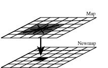
Neighbourhood operations within a window.
Second, the new value of the cell may represent the local drain direction to a neighbouring cell in a local drain direction network over a digital elevation model. These are described in Local drain direction operations.
Third, the new value of the cell may be calculated on the basis of the cells that are on a path starting at a given source cell through consecutive neighbouring cells to the cell in question, see figure below. These operations with friction paths are described in Friction paths. The path represents the shortest distance from the source cell, incorporating friction. Also simply the real distance of the path (for instance the shortest distance to a cell with a garden-restaurant) can be calculated, by specifying a friction of one.
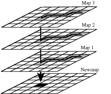
Neighbourhood operations over a path. For each cell the NewMap value is calculated on the basis of Map1, Map2, Map3,... values on a path from a source cell.
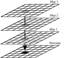
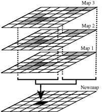
Fourth, the new value of the cell may be calculated on the basis of cells that are upstream from the cell (i.e in the catchment of the cell, see figure below). All these operations use a local drain direction map for hydrologic modelling of transport and accumulation of material in a catchment. These are discussed in Transport of material over a ldd.
Neighbourhood operations within the catchment of a cell. For each cell the NewMap value is calculated on the basis of Map1, Map2, Map3,... values in the catchment of the cell, defined by the local drain direction network.
Fifth, the spatial association may be related to the visibility of cells from a target cell, in an elevation model. These neighbourhood operations for visibility analysis are discussed in Neighbourhood operations: visibility analysis.
Window operations
In a neighbourhood operation within a window, a new value is calculated for each cell on the basis of the cell values within a square window, where the cell under consideration is in the centre of the window.
One can discriminate between two groups of window operations: first each cell value that is calculated may represent a statistical value of the cell values in the window (for instance mean, diversity or extreme values). These operations can also be used to find edges between polygons on a classified map (windowdiversity operator). For these operations the size of the square window can be specified by the user and is not restricted to whole magnitudes of cells.
Second square windows of 3 x 3 cells are used for the calculation of land surface topography, when the PCRaster map is a digital elevation model. These operations include the calculation of slope, aspect and curvature within the window.
Local drain direction operations
A local drain direction network is made with the operator lddcreate on basis of a map with elevation values.
Friction paths
Introduction
This section explains the use of neighbourhood operations for calculating a new value for each cell in the basis of friction cell values on a path between a source cell and the cell under consideration. The accumulation of friction is computed while following a path from a source cell to each cell over a map with frictions (for instance costs). The path that is followed may be determined in two ways. First the paths chosen yield the smallest accumulation of friction. Second the paths may be restricted by the local drain directions on a local drain direction network. In the latter case, the accumulation of friction is calculated for paths in upstream or downstream directions over a local drain direction network.
The operations with friction paths are also used for calculating ordinary real distances over paths (for instance distance to a cell with a railway station). This is done by simply specifying a friction of one.
Operations with friction paths
The principle of accumulation of friction is easily explained by an example of a car driving on an asphalt road for 50 km from point A to point B. This will require x litres of fuel. More fuel is needed if the car travels over a rough surface, such as a sandy track, because the friction will be larger. In general the amount of fuel used is equal to the friction distance, which is the distance to travel (distance) times the amount of fuel used per distance (friction). In this example, the friction depends on the sort of road on which the car has to travel. In an equation:
fuel used = distance * friction
where the fuel used can be regarded as a synonym for the friction distance between point A and B.
All operations with friction use the concept of friction illustrated with the car example. A map with friction cell values is always used to calculate the friction distance between source cells and target cells. The friction values represent some kind of friction per distance unit on the map and may be different between the cells. For instance, the friction may represent the amount of fuel used per unit distance in each cell or the costs of constructing a road per unit distance in each cell. The friction distance (‘amount of fuel used’) between a source cell and a target cell is calculated by travelling over the path between the cells through consecutive neighbouring cells and calculating the total accumulation of friction distance. Each time that is travelled from one cell to the next the friction distance increases as follows: let friction(sourcecell) and friction(destinationcell) be the friction values at the cell where is moved from and where is moved to, respectively. While moving from the source cell to the destination cell the increase of friction distance is:
distance * ((friction(sourcecell) + friction(destinationcell))/2)
where distance is the distance between the source cell and the destination cell. The figure below gives a simple example of a path between a source cell and a target cell travelling through cell A, with a cell length of 4.
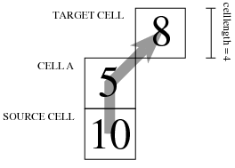
Path from a source cell to a target cell, crossing cell A.
Let the initial friction distance at the source cell be zero. While moving from the source cell to cell A the friction distance increases by:
and when moving from cell A to the target cell in diagonal direction, the friction distance increases by:
So, the total friction distance between the source cell and the target cell is 30 + 36.77 = 66.77.
Of course, on a real map, many possible paths can be found between a source cell and a target cell, through different sets of neighbouring cells. The path which is followed for each target cell can be determined in two ways. The spread operation (and the closely related spreadzone operation) uses the path that results in the shortest friction distance between a source cell and the cell under consideration. For instance, if you use friction values of 1 the real distance to the source cell is calculated which is nearest as the crow flies (in a straight line). Also the path that is followed for each target cell may be determined by a local drain direction map: the operators ldddist and spreadldd (and the closely related spreadlddzone) calculate the friction distance in upstream and downstream direction from the source cells, respectively. The operator slopelength calculates the friction distance in downstream direction from the catchment divide. The above mentioned operations belong to both the group of spread operations and the group of operations with local drain direction maps (with friction like in spread) ldd operations .
Transport of material over a ldd
Introduction
The third group of neighbourhood operations are the operations for hydrologic modelling of transport of material over a local drain direction network. These operations, discussed in the next section, calculate the amount of material transported from upstream cells which is stored in the cell or transported out of the cell.
Operations for transport of material over a ldd
The operations for transport of material over a local drain direction network , can be used for modelling processes that include transport in a downslope direction. In most cases these will be used for hydrologic modelling of water transport or for modelling material transported by water.
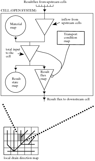
Material transport over a local drain direction network.
The principle of material transport over this drainage network can be explained using the general systems approach. In this approach each cell is an open system. The direction and pattern of transport of material through the map representing a set of systems is given by the local drain direction map: for each cell it defines its upstream neighbours from which material is transported to the cell and its downstream neighbour to which material is transported, see figure above. The state of the cells at the start of the operation is defined by an input map that gives the amount of material that is available for transport. This material map contains for each cell the input of material to the cell at the start of the operation. For instance it may have cell values that represent the amount of rain falling in a cell or the amount of loose soil material that is available in a cell for transport.
The most simple transport operation accuflux does not include conditions that impose restrictions on the amount of material that is transported: all material that flows into a cell flows out of the cell. This can be compared with the transport of water over an asphalt landscape, without infiltration or transpiration. But, in most cases a part of the inflow to the cell will be stored or lost in the cell and only the remaining material will be transported out of the cell. A well known example for such a transport process is the transport of water over an unsaturated soil: only the surplus of the amount of water used for saturation of the soil is transported. Several functions can be used to define this division in transport and storage. These are implemented in the different accu... operations. These operations use a transport condition map , which for each cell contains a value related to the transport function. In the example given above it may contain the amount of water needed to saturate the soil in a cell.
Now we describe what happens to the cells on the map during transport (see also figure Material transport over a local drain direction network.). Transport starts at the cells at the divide of the catchment. For each cell somewhere on the map the total input of material consists of the fluxes of material from upstream cells plus the amount of material at the start of the operation in the cell itself (i.e. the value on the material map). This total input is available for transport. A part of the material is stored in the map and is saved as a (new) result state map layer, the remaining material flows out of the map, to the downstream cell, and is stored as a (new) result flux map layer. The decision about the amount of material that is stored and transported respectively is defined by the sort of accumulation operation that is performed. It is always made on the basis of the cell value of the transport condition map with respect to the total input to the cell.
Area operations
Introduction
The third group of PCRaster operations for Cartographic Modelling includes those that compute a new value for each cell as a function of existing cell values of cells associated with a zone containing that cell, see Area operations. The cell value is determined on basis of values of cells which are in the same area as the cell under consideration.. These operations provide for the aggregation of cell values over units of cartographic space (areas).
The operations are like point operations to the extent that they compute new cell values on basis of one or more map layers. Unlike point operations, however, each cell value is determined on the basis of the several cell values of cells in the zone containing the cell under consideration.
Area operations are also like neighbourhood operations to the extent that they represent operations for two-dimensional areas. But unlike neighbourhood operations, the constituent cells do not conform to any particular ordering or spatial configuration.
Area operations. The cell value is determined on basis of values of cells which are in the same area as the cell under consideration.
Operations over areas
The area operations use a nominal, ordinal or boolean map that contains the separate area classes. For each cel this map identifies the area class to which the cell belongs: cells with the same value on this map are member of a separate area class. These cells belonging to the same class do not need to be contiguous.
For each area class an operation is performed that calculates a statistical value on basis of the cell values of a second input map. This value is assigned to all cells on the resulting map belonging to the class. A wide range of operations is provided such as computation of area averages, determination of the minimum or maximum values within each area or calculation of the sum of the cell values within each area. Generation of a random number for each area is also possible.
Map operations
The fourth group of PCRaster operations for Cartographic Modelling include those that compute one non-spatial value as a function of existing cell values of cells associated with a map, see figure below. The operations are like area operations to the extent that they compute a single value on basis of one or more map layers. Unlike area operations however, the value is determined on basis of all cells in a map.
Map operations.
A non spatial value is calculated on basis of an aggregate value of a map or maps.
For a list of list of operations determine a statistical value on basis of all cell values in a map (for instance the maximum value) or result in a value related to the location attributes of a map, for instance the length of the cells on the map.
Command syntax and script files for cartographic modelling
Introduction
PCRaster distinguishes two kind of operators. The first group of operators is meant for data management (including GIS functions); this is the group of data management operators in Data management . The second group, which is by far the largest, is meant for Map Algebra, Cartographic Modelling and Dynamic Modelling. These are the groups of operators for point operations, neighbourhood operations, area operations, map operations and time operations. Of these, the time operations are only meant for Dynamic Modelling, which will be discussed in the next chapter (Dynamic modelling). All the operations of the second group, except the table operator, use the keyword pcrcalc in the command line (the next section gives the exact syntax). pcrcalc is the program that does these operations. This program is not used for the operators for data management and the table operator.
Both operators that use pcrcalc and operators that do not use pcrcalc can be invoked from the command line by typing one operation after the command prompt. The command syntax of this application of the operator will be explained later in this section (Command syntax)
For Cartographic Modelling, the operations are combined in a script file. The operations in the script file are executed using the same pcrcalc program also used for separate pcrcalc operations. As a result only operations that use the pcrcalc program can be combined in a script file. Operations that do not use the pcrcalc program (data management operations, aguila and the table operator) are not used in a script file. Script files describes how to combine pcrcalc operations in a script file.
Command syntax
Both operations that use pcrcalc as well as operations that do not use pcrcalc can be invoked from the command line, by typing the operation after the command prompt. This section first describes the operations that do not use pcrcalc, second the syntax of the operations that use pcrcalc is given.
Operations that do not use pcrcalc are performed by typing after the prompt:
operator [options] InputFileName(s) ResultFileName(s)
Both the Inputfilename(s) and the Resultfilename(s) are filenames of one or more PCRaster maps, tables or point data column files, depending on the type of operation. If more than one option is given, the options are separated by a space. For instance:
col2map -S -v 3 colfile.txt sodium.map
Operations that do use pcrcalc are given by typing after the prompt:
On MS-Windows:
pcrcalc [options] Result = operator(expression1,..., expressionN)
On UNIX:
pcrcalc [options] ‘Result = operator(expression1,..., expressionN)’
where operator is one of the pcrcalc operators and expression1,..., expressionN are PCRaster maps or pcrcalc operations resulting in a PCRaster map with a data type that applies to the operator. In some cases a single number may be filled in for the expressions, see below. Result is a PCRaster map. Whether quotes are used or not depends on whether the command line contains a command shell special symbol. Without quotes a special symbol in the command is interpreted as having the meaning defined by MS-Windows or UNIX. In UNIX the = sign is a special symbol. As a result quotes must be used in UNIX for all pcrcalc operations. No special symbols of MS-Windows are used in pcrcalc operations except the ‘<’ and ‘>’ symbols in a few operations. So in general quotes are not needed in MS-Windows. If the command contains a ‘<’ ‘>’ the quotes must be applied in the same way as it is (always) done in UNIX.
The use of pcrcalc operations for expression1,..., expressionN allows for nested operations. The number of operations used to define these expressions (so called because these may be expressions that result in a PCRaster map) is practically unlimited. For each separate statement, pcrcalc is typed only once, at the start of the line. For instance:
pcrcalc AspectTr.map = if(VegHeigh.map gt 5 then aspect(Dem.map))
uses the if then, gt or > and aspect operators. Remember that the nested operations must result in correct data types. For instance, in the operation given above, the gt operation results in a map of boolean data type needed for the first expression of the if then operator. The second expression of the if then operator (typed after then) may have any data type, in this case it is directional.
Numbers and data types
Using a plain number (giving no data type specification, for instance the ‘5’ in the operation given above) for an expression is possible if it is taken into account that the number that is filled in must be in the domain of the data type that is needed for the expression under consideration. For instance a value 8.7 cannot be filled in if a nominal data type is needed . In addition, a plain number may not be used if for determination of the data type of Result the data type of the expression for which the number is filled in is needed. For instance the following operation is not correct:
pcrcalc Friction.map = if(Boolean.map then 1 else 2)
because the data type of Friction.map cannot be determined on basis of ‘1’ and ‘2’. In this kind of cases one of the data type assignment operators must be used; the correct operation for assigning a scalar data type to Friction.map is:
pcrcalc Friction.map = if(Boolean.map then scalar(1) else scalar(2))
Script files
Simple script files
Most geographic analyses contain a number of steps. PCRaster can be used to write down these steps in one script file and execute these steps sequentially. The thus created scripts are called Cartographic Models. A script contains a list of pcrcalc operations which describe the Cartographic Model. During execution of a script these operations are performed consecutively, from top to bottom in the script. Two layouts of a script can be used: with or without the binding section. First we describe how to use the plain script without the binding section. In the second part of this section we describe the script with binding section.
The script without binding has the following layout:
operation of calc;operation of calc;......
The script contains only pcrcalc operations, other operations which do not use the pcrcalc program (for instance table) cannot be used in a script. Each pcrcalc operation is typed on a separate line, omitting the word pcrcalc from the operation and terminated with a semi colon (;). On the right side of the = sign, an operation may use a file (a PCRaster map or for the lookup operation a table) that is present in the database, a file that is defined in the script or a plain number. The result (on the left side) of an operation is always a PCRaster map. Remark lines are preceded by a # character: everything typed on a line after this character is ignored and has no effect on the function of the model. An example of a script file is:
# this is a cartographic modelling script file
Friction.map = lookupscalar(Friction.tbl,LandUse.map);
Friction.map = 2.5 * Friction.map;
CostDist.map = spread(Start.map,0,Friction.map);
The first line is a remark, it is ignored by PCRaster. In the second line the script generates a map Friction.map with the lookupscalar operator from the files friction.tbl and LandUse.map, which must be present in the database. In the third line the Friction.map is multiplied by 2.5. In the fourth line CostDist.map is generated from the Friction.map defined in the script and Start.map already present in the database. In the fourth line the Friction.map is taken resulting from the last operation defining this map, i.e. the values resulting from the operation in the third line.
Normally, without using report keywords, all resulting map values (on the left side of = sign) at the end of running a script are stored in the database, saving for each PCRaster map the last definition. In the example given above the Friction.map and the CostDist.map are stored in the database under these names. The last definition of Friction.map is stored, resulting from the third line. Alternatively specified results can be stored by typing the report keyword before a limited number of operations in the script. In that case, only the result of the operations preceded with report are stored. A certain resulting map name can be reported only once. For instance:
- ::
- # example of a script file Friction.map = lookupscalar(Friction.tbl,LandUse.map); Friction.map = 2.5 * Friction.map; report CostDist.map = spread(StartMap,0,Friction.map);
This script only stores CostDist.map in the database. If in addition the operation in the second line was also be preceded with report, then the values of the Friction.map resulting from the operation in this second line would be stored too. If the operation in the third line would be preceded with report, the values of the Friction.map resulting from the operation in this third line would be stored. Note that Friction.map may not be reported both in the second and the third line: this would result in reporting one map name twice in a script, which is not allowed.
The ascii formatted script can be created with a text editor or with a word processing program storing the file as ascii text. A script is executed by typing after the command prompt:
pcrcalc -f ScriptFileName
where ScriptFileName is the name of the ascii formatted script file.
Script files with binding section
An extension to the plain script is the script with a binding section . In a plain script, files (PCRaster maps or tables) are directly linked to these in the PCRaster database: the names used in the script correspond with these in the database. A script with binding definitions allows for different names in the model part of the script. The binding binds the names of the files in the script to the names of the files in the PCRaster database. Often you may want to run a Cartographic Model script a number of times, each time with a different set of data files and with a different set of resulting files. In most cases, these data files are used a large number of times throughout the program. Using the binding, you only need to fill in the names of the files you want to use as input names and output names for the model run in the binding section, without changing all the file names in the rest of the script. Both file names used as input files for the model and names that are stored in the database during a model run with the report keyword may be given in the binding section.
A script with a binding definition is divided up in two sections: the binding section and the initial section. It has a structure as follows:
bindingbinding statement;... ...initialoperation of calc;operation of calc;... ...
The binding section starts with the section keyword binding. Each line after this keyword contains one binding statement. Each statement gives a name for a PCRaster map or table in the script that is different from the file name of that variable in the database. Both file names used as input files for the model and names that are stored to the database during a model run with the report keyword may be given. The name of a file in the database is bound to its name in the model with the following statement:
NameInModel = databasefilename;
where databasefilename is the file name under which the variable is available in the database or will be stored to the database and NameInModel is the name used for the variable throughout the script.
Alternatively, a constant value can also be assigned to a PCRaster map variable. This applies only if ModelName is a PCRaster map which is an input to the model:
NameInModel = value;
where value is a number; NameInModel has this value throughout the Cartographic Model; its value cannot be changed. It has no data type attached to it. Attaching a data type to the PCRaster map NameInModel with a constant value is done by one of the data type assignment operators. We advice to specify the data type always because most operations need to know the data type of the maps used. An example that assigns a boolean data type to NameInModel is:
NameInModel = boolean(1);
The data type assignment operators are the only pcrcalc operations that can be given in the binding section, other operators cannot be used.
Not all variable names need to be defined in the binding section; as said above, the filenames of the variables in the database can also be used in the script.
The second section of a script with binding section is the initial section. It starts with the initial section keyword. The following lines contain the Cartographic Model, formatted in the same way as the plain script. Also the use of reports and # characters for remarks corresponds with the plain script. Using a binding, the plain script with a report might look like this:
Example of a cartographic modelling script file
# Example of a cartographic modelling
# script file with binding and initial section

binding
 # this is the binding section
 FrictionTable = Fr12.tbl;
 StartMap = Station.map;
 CostDistanceMap = CostRun1.map;

initial
 # this is the initial section
 FrictionMap = lookup(FrictionTable,LandUse);
 FrictionMap = 2.5 * FrictionMap;
 report CostDistanceMap = spread(StartMap,0,FrictionMap);
The initial section has not been changed. The binding section binds the Station.map, already present in the database, to the name in the model StartMap. The table Fr12.tbl in the database is used as FrictionTable. LandUse is not bound in the binding section; as a result it must be present in the database as a map with name LandUse. The report CostDistanceMap is stored in the database under the name CostRun1.map.
A script with binding section is also ascii formatted text. It is executed in the same way as the plain script.