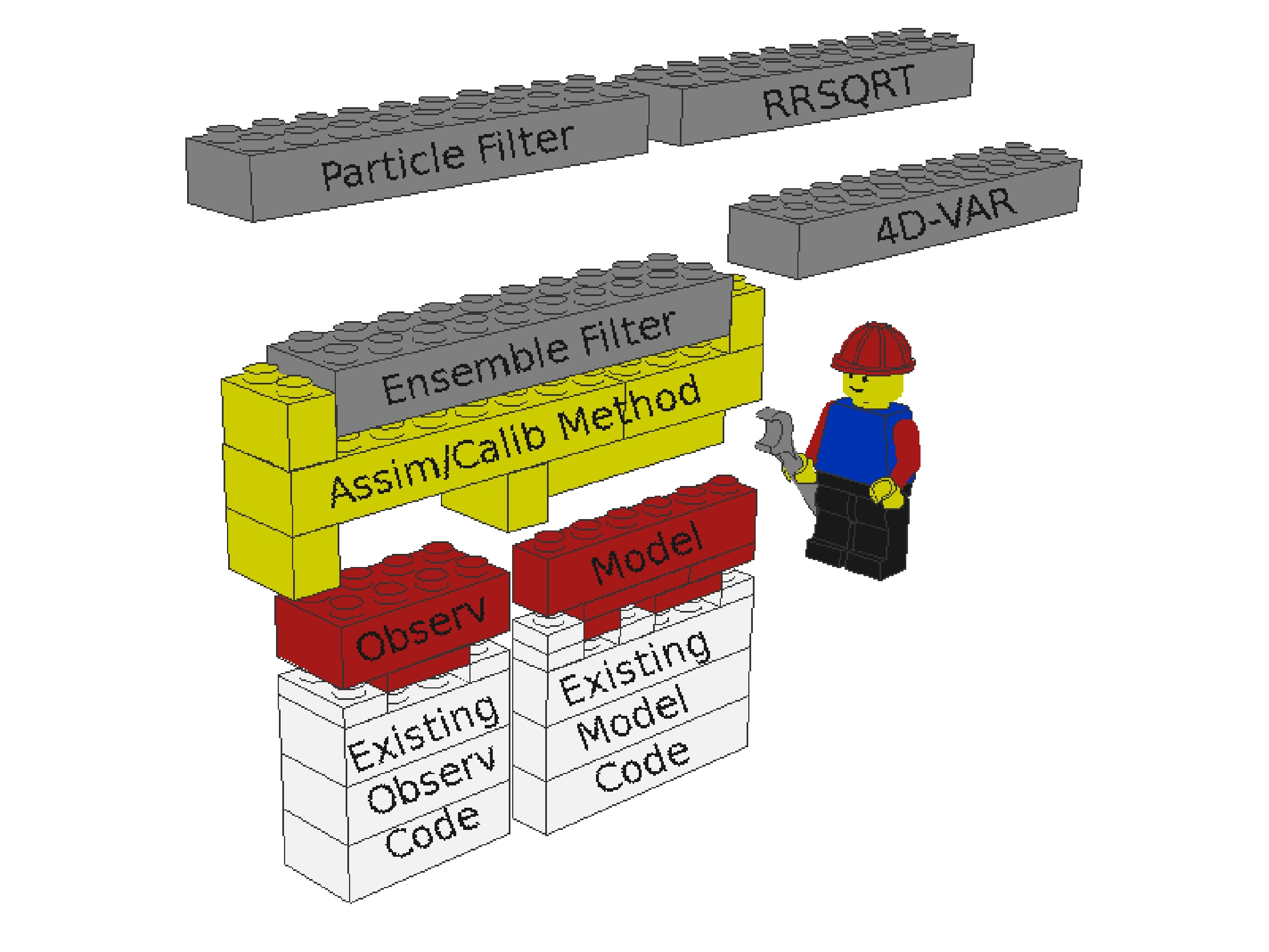
 Basic design of the OpenDA system. Model and observation components (red/white bricks) are plugged into the core of the
OpenDA environment (yellow bricks), and can then exploit the available data-assimilation methods (grey bricks).
Basic design of the OpenDA system. Model and observation components (red/white bricks) are plugged into the core of the
OpenDA environment (yellow bricks), and can then exploit the available data-assimilation methods (grey bricks).
The basic design philosophy of OpenDA is illustrated in the figure. The key elements in this picture are:
The figure intends to illustrate a number of important points:
In OpenDA two components are defined: the OpenDA model component and the OpenDA stochastic observer component. There can be multiple instances of each of these components, each with their own set of data. The set of routines to manipulate the data is called the interface of the component. (Note: the terminology used in OpenDA with respect to object orientation is described in the paragraph about OO terminology).
OpenDA defines the interface of the OpenDA model component. This consists of the list of methods/routines that a model must provide. Examples are "perform a time-step", "deliver the model state", or "accept a modified state". This interface of the model component is visualized through the shape of the empty space in the yellow bricks in the figure above.
Usually, existing model code does not yet provide the required routines, and certainly not in the prescribed form. Therefore some additional code has to be written to convert between the existing code and the OpenDA model components interface. This is illustrated in the figure using red and white bricks: the white bricks stand for the original model code, whereas the red bricks concern the wrapping of the model in order to provide it in the required form.
OpenDA similarly prescribes the interface of the OpenDA observation component. This is visualized using a second empty space in the yellow bricks in the Lego figure. For using OpenDA for your model you must fill in this part, by wrapping the existing code for manipulation of your observations and providing it in the required form.
The data assimilation algorithms in the Lego figure cannot (yet) be seen as instances of another component. For now they are merely routines that implement different data assimilation techniques with the elements provided by OpenDA as the building blocks (models, observations, state vectors etc.). There is however a convergence to a fixed form, a more or less standardised argument list for data assimilation algorithms, such that eventually these may be turned into a well-defined component.
The basic design of OpenDA may seem disadvantageous at first, because it appears to require additional programming work in comparison to an approach where data assimilation is added to a computational model in an ad-hoc way. This is usually not the case. Most of the work in restructuring of the existing model code is needed in an ad-hoc approach too. This is because data assimilation itself puts requirements on the way in which the model equations are implemented in software routines: one must be able to repeat a time step, to adjust the model state, to add noise to forcings or the model state, and so on, which is often not true for computational models that are not implemented with data assimilation in mind.
The basic design does have a huge advantage over an ad-hoc approach for adding data assimilation to an existing program. It is that the different aspects of a data assimilation algorithm are clearly separated. The algorithmics of the precise Kalman filtering algorithm used are separated from the noise model, which in turn may be largely separated from the deterministic model and the processing of observations. This makes it easy to experiment with different choices for each of the parts: adjusting the noise model, adding observations, testing another data assimilation algorithm and so on. This is the major benefit of using the OpenDA approach.
Contents of the OpenDA toolbox
The yellow part in the Lego figure provides the infrastructure needed for connecting generic model and observation components to
generic data assimilation methods. We go into the contents of this part in order to gain a better insight in the structure and
working of the OpenDA system.
The non-Java components of OpenDA are implemented using non-object oriented programming languages, particularly using Fortran and C. (One reason for this is to avoid difficulties when connecting model software that is written in Fortran and C, another motivation is the experience with Fortran and C of the original developers). However, OpenDA does use ideas from object orientation. In particular the following terminology is used:
Whereas the current OpenDA software and documentation often uses the word "component", Wikipedia ("Component based software engineering", "Class (computer science)") suggests that "class" would be more appropriate in most cases, with exceptions for the model and observer components. We suggest to adhere to the terminology introduced here.
| OO Language | OpenDA |
| String s1, s2; | CTA_String s1, s2; |
| char cstr[100]; | char cstr[100]; |
| S1 = new String; | CTA_String_Create(&s1); |
| s2 = new String; | CTA_String_Create(&s2); |
| s1.Set("hello "); | CTA_String_Set(s1,"hello "); |
| s2.Set("world"); | CTA_String_Set(s2,"world"); |
| s1.Conc(s2); | CTA_String_Conc(s1, s2); |
| s1.Get(cstr); | CTA_String_Get(s1, cstr); |
| free(s1); | CTA_String_Free(s1); |
| free(s2); | CTA_String_Free(s2); |
As an example we consider the support for strings in OpenDA. A class CTA_String is provided for them. It is a simple container for character strings, which is primarily introduced to shield the difficulties of sharing text strings between Fortran and C. The operations provided for OpenDA strings are to create a new instance, set its value, concatenate strings, retrieve its value, and cleanup a string when it is not needed anymore. A piece of code using this class is presented in the table above.
Another basic class is the OpenDA time class, which provides a uniform way of handling time. The class registers a time span (interval) and optionally contains a time step attribute. It may be extended in a future version with various time scales and representations, time zones, etc..
A third basic building block is the OpenDA vector class, which contains a dimension (length), the data type of the vector elements (equal for all elements), and the values of the vector elements. An advantage of incorporating a vector class in OpenDA is that it provides a generic entity on which data assimilation algorithms can be based, without unnecessarily restricting oneself to the actual data type being used. Further, one can choose to provide different implementations (derived classes) of the vector class, for instance a distributed vector (for parallel computing, sparse vector (if a significant amount of zeros may occur, or using an optimized BLAS version.
An important class in the OpenDA toolbox is the OpenDA tree. It is a generic class for grouping and structuring of data. It may be compared to a "struct" in C or derived type in Fortran. One notable difference is that a OpenDA tree is a dynamic entity: additional items may be added at run-time, with the names of the items provided as string arguments to the creation routines. Therefore a OpenDA tree may also be compared to a file system; nodes contain OpenDA trees (like directories), and leafs contain other OpenDA objects (like files).
A special kind (derived class) of OpenDA tree is the OpenDA tree-vector. It is a OpenDA tree that contains only OpenDA vectors as leaf elements. Of course it provides all the operations that a OpenDA tree class provides. Further it supports the operations that a OpenDA vector is able to perform. The OpenDA tree-vector is important for instance for describing a model state. In data assimilation one must be able to combine different model states much like vectors can be combined. However, representing the model state by a single vector is a severe restriction for many computational models. It is preferable to be able to distinguish different parts of the state, and sometimes needed to distinguish elements with different data types. Furthermore the hierarchical nature of the OpenDA tree-vector supports composition of larger models states out of smaller ones as described later on.
OpenDA primarily uses the XML-format for input/configuration-files. There are several facilities for quickly reading such input-files. OpenDA trees (and tree-vectors) may be written to and read from XML-files as well.
Interfaces are defined to the OpenDA classes for use in Fortran and C/C++. An interface for Java is defined separately in the OpenDA project. This allows data assimilation algorithms to be implemented in Java, and be used together with model components made in Fortran and C.
The OpenDA toolbox can be installed on various Linux and Unix-platforms using the well-known Automake facilities. For the Windows platform project files for Microsoft Visual Studio are provided.
The OpenDA Application script uses an XML-file to create new OpenDA applications. The XML-file defines the three main ingredients:
Within the field of data assimilation a distinction between off-line and on-line assimilation methods can be made. Off-line data assimilation concerns model calibration, i.e. optimizing the parameters of a model such that the best fit with a set of observations is obtained.
In these methods the initial value of the model state may be considered as an input parameter of the model as well. This links the 3D-VAR and 4D-VAR variational approaches to the off-line methods listed above.
On-line or sequential data assimilation methods consist of a cycle of forecast and analysis steps, where the methods assimilates the data each time that observations become available. Optimal interpolation methods and Kalman filtering methods fall into this class.
Data assimilation techniques will have to access the model state. This cannot be done directly. A model may use its own representation of the state. The interface of the OpenDA model component however requires that a model be able to provide a copy of the state in a OpenDA tree-vector, and that linear operations on a state-vector can be performed.
Linear operations on the model state are an important aspect of the interface of the model component because these operations are used frequently in data assimilation algorithms, and because the implementation may be dependent on the actual model that is implemented. For instance a model may require positivity of specific quantities that it computes (e.g. waterdepth in a flow model), such that blindly combining two state-vectors may give inappropriate results. Therefore a more careful combination recipe may be implemented by the model itself.
One place where this idea is given concrete form is in the concept of model builders. A model builder is more or less a template for creating new native model components. It fills in as many of the routines that must be provided, such that setting up a new model component is greatly simplified. Once one is up and running one can then tune the implementation to ones own ideas.
Note that parallelization of data assimilation methods can often be achieved in different ways. A data assimilation algorithm often contains multiple model computations that may be performed in parallel, and each model computation itself may be parallelized too. The former approach to parallelization is called "mode-parallel". This name stems from the term "error modes" that may be used for different model instantiations in certain Kalman filtering algorithms. The latter approach using parallelization of the model computation itself is called "space-parallel", which indirectly refers to the domain decomposition approach. The two approaches may be combined as well, which gives a "mode and space-parallel" approach.
The parallel model builder is primarily concerned with space-parallelization. Mode-parallelization is already provided by the sp-builder ("using OpenDA, you get mode-parallelization for free"). It is provided by the parallel model builder as well, which yields the mode+space parallel approach.
The architecture used by the parallel model builder is to use an SPMD-approach ("single-program, multiple data"), i.e. to start the main OpenDA-application (executable) multiple times. Within the group of processes that is created in this way, the first one acts as the master process. This process performs the data assimilation algorithm. The other processes perform the model computations.
Computational models that use a master-worker approach for their parallelization may fit well into this approach. The master process of the original computational model may be integrated with the OpenDA master process. The subroutines that are required by the OpenDA model components interface may be filled in using the routines of the model's master process. This may be achieved well with the sp-builder.
The parallel model builder is mainly concerned with computational models that are parallelized using a worker-worker approach, e.g. using domain decomposition, where each computational process solves a different part of a global domain.
The routines that are specified in the OpenDA model components interface, like "perform a timestep", are implemented differently in the master and worker processes. In the master process, these routines consist of sending MPI messages to the worker processes, and waiting for the corresponding results. The results are joined together more or less the same as when different sub-models are combined into a composite model.
The worker processes read a configuration file from which they learn about their role in the global computation. Then they go into "worker-mode". This consists of an indefinite loop, waiting for MPI messages, and calling the appropriate model routines. The model routines are implemented just like for a sequential model. One notable difference is that these routines are called in all worker processes simultaneously, such that communication between the workers may be used.
The parallel model builder provides the infrastructure needed for setting up this scheme. It provides the model routines for the master process and the worker mode for the OpenDA main program. The model engineer just has to provide the model routines for the worker processes.
The Stochastic Observer is the OpenDA component that holds an arbitrary number of observations. It may be instantiated multiple times.
A stochastic observer may be queried for a selection of the observations that it holds. For instance the observations within a given timespan may be requested, for a selected set of "stations", or that measure a specific quantity. Such a selection may be used to create a new stochastic observer object.
The stochastic observer further takes care of computing predicted values at observation locations. This concerns the observation relation that is used in data assimilation algorithms: the model state is interpolated and/or converted to the observation location and observed quantity. For this the implementation of a stochastic observer must know the structure of a model state vector, the meaning of its components, and the procedures available for spatial and/or temporal interpolation. For this a stochastic observer contains a substantial application dependent part.
OpenDA provides default implementations of the stochastic observer and observation descriptions. In this default implementation observations are stored in an SQLite3 database. The database contains two tables, "stations" and "data" for time-independent and time-dependent information respectively. This default implementation provides a basis for setting up ones own observation component. It should grow over time with features that are relevant to different computational models.